demo
The classifier over a day of frames, spots turning red as cars arrive, green as they leave.
the idea
Detecting free parking usually sounds like object detection: find every car in a photo of a lot. But if the camera is fixed, the spots never move, their locations are known in advance. That one observation collapses the problem: instead of detecting cars anywhere in the frame, I only need to look at each known spot and answer a single binary question: occupied or empty?
data and baseline
I used PKLot: ~695,000 pre-segmented parking-space crops from three lots (UFPR04, UFPR05, PUCPR) across sunny, rainy, and overcast weather, each labelled empty or occupied.
My first action was to explore the data. The classes are 51.5% empty / 48.5% occupied (358,071 vs 337,780; my count matched the published figure to within 0.007%). That near-balance sets my majority-class baseline at 51.5%, the score of a model that blindly guesses "empty." Every accuracy number later is measured against that 51.5%. (Balanced data also meant I didn't need resampling or class weights)
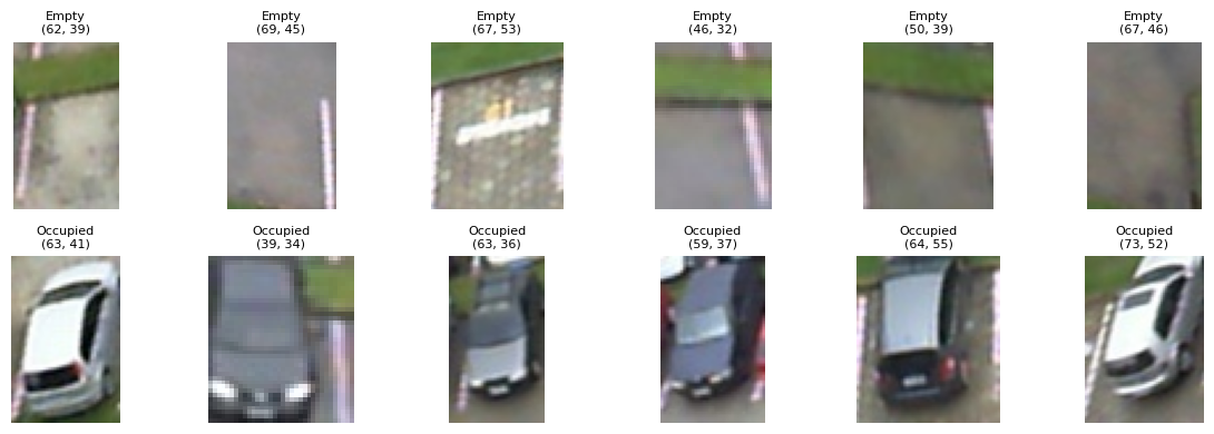
Sample crops. Top row: empty spots (asphalt, grass, painted lines). Bottom: occupied. The classes are clearly separable by eye, the signal exists. Note the crops are all different sizes (titles show pixel dimensions), which forced a resize step later.
I developed on a balanced 2,000-per-class sample from one lot (UFPR04) and left the other two lots untouched. I wanted the other lots to test generalization, and early peeking would cause data leakage and inaccurate results.
feature engineering
A model needs a fixed-length numeric vector, and the crops are all different sizes, so step one was resizing every crop to 64×64. (Why square, accepting mild distortion? Every crop is distorted the same consistent way, so the model isn't confused, and padding to preserve aspect ratio adds complexity for no benefit here.) Then two complementary feature types:
HOG (Histogram of Oriented Gradients) captures shape: it discards color and keeps only the direction and strength of edges. A car has hard edges, a windshield line, body-panel curves; empty asphalt is flat.
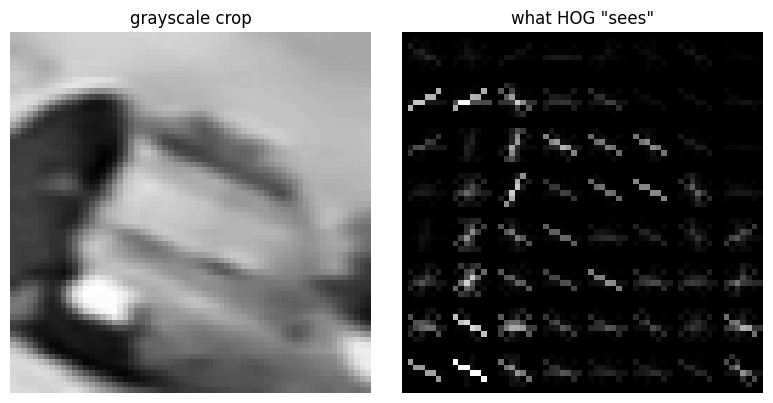
Left: a grayscale crop. Right: what HOG "sees". Gradient orientation and strength per cell. The car's edges light up as bright structure; flat regions stay dark. It's about shape, with all color thrown away.
A color histogram captures color. I chose HSV rather than RGB because HSV separates brightness (which shadows change) from hue and saturation, making it more robust to lighting.
Going in, I had a hypothesis I wanted to test: shape (HOG) will dominate color, because cars come in every color, a grey car is asphalt-colored, a black car shadow-colored, so color seemed like a weak signal. Alongside, training and evaluating my model, I wanted to test this hypothesis.
two models
After a stratified 80/20 split and feature scaling, I trained two models. I scaled after splitting (to avoid my test set being leaked), fitting the scaler on the training set only.
I trained logistic regression first, the simplest sensible model, and a probe: if a purely linear model scores well, the classes are linearly separable in this feature space. Then a random forest, for non-linear interactions and, later, feature importances.
Both scored 99.62%, identical to four decimals. It was a bit anticlimactic honestly, but it did answer the question of whether the extra model complexity bought me anything: no. The feature engineering did the work; a straight-line boundary was already essentially optimal.
The 99.62%: it's in-lot (same camera as training), on one lot, and because PKLot is time-lapse, it is often a near-duplicate crop, minutes apart in both train and test, so the 99% is a bit optimistic. It's also consistent with the ~99% the original PKLot paper reports for hand-crafted features, so at least we're consistent here.
interrogating the model
Confusion matrix & precision/recall. Both models missed only ~3 of 800 crops, with ~1.00 precision and recall on both classes.
Cross-validation. A single split has no error bar. Across five stratified folds, logistic regression averaged 0.9978 (±0.0013) vs the random forest's 0.9938 (±0.0036). So logistic regression was marginally better and ~3× steadier. This means "stable in-lot" and "strong to a new camera" are different properties.
ROC-AUC. Both ~0.9998: near-perfect, threshold-independent separation.
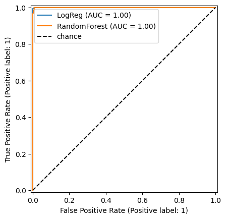
Both models' ROC curves hug the top-left corner (AUC ≈ 0.9998). Near-perfect class separation in-lot.
Feature importance: my hypothesis. I tested "shape dominates color" three ways and got three different answers:
- Impurity importance suggested the opposite, color looked more important.
- Permutation importance returned ~0 for everything — not a bug, but a signal my features are heavily redundant (shuffling one feature does nothing because correlated neighbors cover for it).
- Ablation (training on each feature group alone) was the cleanest test: HOG-only 99.0%, color-only 99.1%. A statistical tie under cross-validation, with the lead even flipping between runs.
So my hypothesis was wrong, but so was the naive "color wins." The truth: shape and color are equally informative, each nearly sufficient alone, but they still compliment each other (together they beat either, that's why using both is justified). The real lesson is methodological, using only one feature importance method would've given me a wrong answer, it's important to triangulate.
Failure analysis: looking at the mistakes.
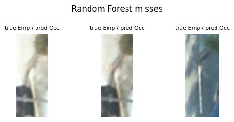
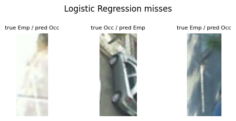
The crops each model got wrong, with true vs predicted labels. These sort into named failure modes rather than random errors.
The 3 errors per model sorted into crop-boundary intrusion (a neighbor's car bleeds into the crop, a limitation of the fixed-crop design, not the model), painted-line ambiguity, and overexposure. Only one crop fooled both models:
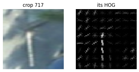
The one crop both models missed. HOG-only classified it "occupied" (0.56); color-only correctly said "empty" (0.44). The shape features were fooled, consistent with the white parking line's strong gradient reading as a car edge, while color wasn't.
The big-picture takeaway: at 99.6%, the remaining errors are largely irreducible on this feature set. Due to the crops and some ambiguity in the way cars can be parked, this isn't something more hyperparameter tuning would fix.
the real test: generalization to a new camera?
Everything above says the model is excellent on the camera it trained on. The new question: did it learn "what a car looks like" (transferable), or memorize UFPR04's scenery? So I trained on UFPR04 and tested on two cameras it had never seen.
| Test lot | Logistic Regression | Random Forest | (in-lot ≈ 99.6%) |
|---|---|---|---|
| UFPR05 | 71.4% | 89.2% | 99.6% |
| PUC | 93.3% | 95.1% | 99.6% |
The random forest generalized better than logistic regression, reversing the in-lot ranking, because a single global linear boundary gets shoved out of place by a distribution shift while the forest's local regions resist. And UFPR05 was harder than PUC, the opposite of what I'd guessed from how different the lots look to a human. It was interesting to witness how perceptual similarity isn't feature-space similarity.
How it fails. Every confusion matrix failed the same way: biased toward "occupied." Occupied recall stayed ~98–100%; empty recall collapsed (as low as 44%). The reason is clean and ties back to the feature story: "occupied" is lot-invariant, a car looks like a car anywhere, while "empty" is lot-specific, each lot's bare ground, asphalt tone, and angle differ (based on camera angle, lighting, weather). On a new camera, unfamiliar empty ground stops matching the memorized template and drifts toward "occupied." The color features that recognized UFPR04's consistent empty signature are what fail to transfer.
But is it lost signal, or a misplaced threshold? I checked ROC-AUC, which is threshold-independent, and it stayed high even where accuracy fell (UFPR05 LR: AUC 0.94 but accuracy 0.71). High AUC + low accuracy means the model still ranks crops correctly, the classes are separable, but the fixed 0.5 decision threshold, calibrated on UFPR04, sits in the wrong place for a new camera's shifted scores. So most of the loss is calibration, not lost signal.
There's a practical upside to which direction the errors fall. In a real garage the two mistakes aren't equally bad. The costly one is telling a driver a spot is free when it's actually taken: they drive over, find it occupied, and stop trusting the system (in my labels, a false negative: predicting empty when it's really occupied). The harmless one is the reverse, marking a free spot as taken, because the app just doesn't offer that spot, the driver parks elsewhere, and no one is inconvenienced (a false positive: predicting occupied when it's really empty). It's better the system lean toward "occupied": to skip a free spot than send someone to a full one.
To prove it, I recalibrated the threshold on a small labelled sample from each new lot and evaluated on the rest.
| Case | default @0.5 | recalibrated | threshold |
|---|---|---|---|
| UFPR05 · LR | 71.4% | 85.4% | 0.99 |
| UFPR05 · RF | 87.7% | 95.7% | 0.65 |
| PUC · LR | 94.2% | 96.9% | 0.98 |
| PUC · RF | 95.7% | 98.3% | 0.62 |
Recalibration recovered most of the loss with no retraining, and matched the best-possible threshold almost exactly. So a small labelled batch from a new camera is a deployable fix. Every calibrated threshold sits above 0.5, compensating for the upward score drift.
real-time
Finally, the whole pipeline running live on full-lot frames. Using the fixed-camera premise, spot locations defined once, reused every frame, the system crops each spot, classifies it, and annotates the frame.

Each spot is perspective-warped from its rotated outline into an upright crop, so inference crops match the training distribution (a mismatch here would hurt accuracy.
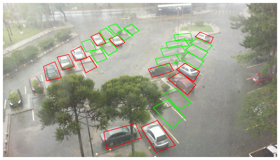
A full frame with per-spot predictions: red = occupied, green = empty. (This is a rainy frame, the model handles wet conditions it saw in training.) Notice a false-negatve classification.
The pipeline runs at 57 FPS (17.5 ms/frame) on a CPU, no GPU. Parking occupancy changes over minutes, so that's roughly 100× more throughput than the application needs.
reproducibility
Data comes from the PKLot database via a single documented download (the ~5 GB of images are git-ignored and fetched, not committed). Every number here was measured, not estimated, with fixed random seeds for reproducible splits and samples.
Tools: NumPy, Matplotlib, OpenCV, scikit-image, scikit-learn. A classical ML project.