the idea
CBC reports, "more than 3.8 million hectares of land — including over 730,000 hectares in Ontario alone — have burned across Canada this year."1
With the growing dangers and risks of wildfire spread, it's becoming increasingly detrimental for the survival of our trees, to be able to detect wildfire spreads. I took it as a challenge to solve the rising global issue by building my own CNN and comparing against transfer learned CNNs to compare accuracy, precision, and other metrics.
Every "scratch CNN vs transfer learning" comparison I'd read ends the same way: transfer learning wins, use transfer learning. Fine. But why does it win? Is it the pretrained weights, or is it just that people compare their small hand-built model against a much bigger architecture and credit the win to pretraining?
That's another question I wanted to answer properly: build a CNN myself, benchmark it against a pretrained backbone, and design the experiment so I can tell which factor caused which part of the gap.
I scoped my first task to discovering that the benchmark I'd picked can be beaten by a model that never opens an image file.
exploring before training
I used The Wildfire Dataset2: 2,700 images labelled fire or nofire, pre-split into train/val/test, backed by a published paper. The obvious move is to load it and start training. I explored it first, a valuable habit from my parking occupancy classifier project3 that I picked up.
My first action was a file count. It came back at 2,699. One of the "images" was `desktop.ini`, a Windows folder-settings file that got swept up when someone uploaded the directory. Harmless, but it told me the published counts hadn't been re-derived from the actual archive.
Then I printed some filenames. I printed the first eight names from each folder, sorted. They all looked like this:
11713547914_dd11630b77_o.jpg
18983401442_9023bb668c_o.jpg
Flickr photo IDs. Flickr assigns IDs roughly sequentially at upload, so near-consecutive IDs mean one photographer's session, which for a fire dataset means the same fire, possibly split across train and test.
Then I counted how many files actually matched that pattern. 1,187 of 2,699.
Sorting filenames as strings puts digit-leading names first, because `'1' < 'a'`. My "sample" was a sample of exactly the subset that happened to be named the way I assumed. The other 56% looked like this:
balazs-busznyak-ZGmQ4qVsaTc-unsplash.jpg
maciek-sulkowski-Bktevt0SwQw-unsplash.jpg
Unsplash. Two sources. And in a shuffled sample of thirty Unsplash files, twenty-nine were labelled `nofire`.
Never take the first N of anything as a sample. It's ordered by something, and that something is rarely random. This trap caught me more times than I'd like to admit in this project.
the number that changed the project
I crosstabbed source against label:
| source | fire | nofire |
|---|---|---|
| Flickr | 989 | 198 |
| Unsplash | 56 | 1,456 |
So consider a "model" implementing this rule: if the filename ends in `-unsplash.jpg`, predict no-fire; otherwise predict fire. It doesn't need parameters, doesn't look at pixels; it never decodes a single image.
It scores 92.4% accuracy on the dataset's official test split. The majority-class baseline, always guess the more common class, is 61.2%.
This isn't an accusation of anything. It's a consequence of collection bias: fire photographs came from Flickr and government agencies, forest scenery came from Unsplash. But it means the two classes differ in photographic style, colour grading, saturation, composition, gear, not only in whether something is burning.
This is what people mean by "shortcut learning." A model finds a signal that's easier to learn than the one you wanted, and that happens to correlate with the label in my data. The canonical example is Zech et al. (2018)4: chest X-ray models that appeared to detect pneumonia were partly detecting which hospital's scanner took the image, because sicker patients get portable scans. The model wasn't reading lungs. It was reading metadata baked into the pixels.
Same process here. Fire is orange and dramatic; stock photography is polished and saturated. A CNN will happily learn "polished" because polished is easier.
Frustratingly, the implication I can make is that a notebook reporting 96% on this benchmark has told me almost nothing, because it's barely cleared a filename regex.
keep it or switch it?
This should be strong evidence to why data research is important. I really wanted to move on and just find a cleaner dataset, but the reason for keeping this dataset generalizes.
Every scraped image dataset has this problem. Positives and negatives get collected from different places because that's the easy way to collect them. If I switched, the realistic outcome wasn't that the problem would vanish, it was that I wouldn't find it, because I'd have just spent a day switching and would be impatient to train something.
So like any good data scientist, I asked myself: is this flaw fatal or bounded? Fatal means my central claim becomes unmeasurable. Bounded means I can build an evaluation that neutralises it.
I had 198 Flickr non-fire images. That turned out to be enough.
building an honest evaluation
I rebuilt the split from scratch with two properties.
Group-aware. The official split is random by image, but images come in groups, either Unsplash photographers or Flickr upload sessions. Half the dataset sat in groups across a split boundary. A "group split" means the whole group goes to one side; I never train on one photo of a scene and test on another.
I checked how much that actually mattered. Using perceptual hashing, reducing each image to a 64-bit fingerprint of its low-frequency structure, so crops and recompressions barely change it, I measured every test image's distance to its nearest training image, and calibrated the "same scene" threshold by eyeballing pairs band by band. 3 of 410 test images (0.7%) were near-duplicates, stable across thresholds of 5, 8 and 11.
Stratified on source × class, with Flickr negatives deliberately concentrated in test. 95 of them, against 24 in the official split.
This second choice is my whole design. It produces a source-matched slice: 247 test images, 152 fire and 95 no-fire, all from Flickr. On that slice the filename rule scores exactly 0.500, pure chance. A model can only beat chance there by looking at the picture.
And the slice is also the hard part of the dataset, because the Flickr negatives are the confounders the paper purposefully collected: sunsets, sun glare on water, fog, low cloud. Images that look like fire and aren't.
Every headline number in this project is measured on that slice.
a note on the metric
I report ROC-AUC rather than accuracy. This means, if you pick one fire image and one no-fire image at random; AUC is the probability the model gives the fire one a higher score. 0.5 is a coin flip, 1.0 is perfect ranking.
The reason I prefer it here is that it doesn't depend on where I put the decision threshold, and my classes are imbalanced differently on different slices.
It's also worth knowing that AUC is not immune to the shortcut. The filename rule scores 0.828 AUC on the full test set. It's only on the source-matched slice that it drops to 0.500. Choosing a threshold-free metric doesn't save me from a contaminated test set, choosing a clean test set does.
three models, not two
The comparison I'd planned was: my hand-built 94k-parameter CNN versus a fine-tuned EfficientNet-B05.
But while building the architecture of my hand-built neural network, I realized there's two ways that which these models can differ; 1. architecture and 2. pretraining.
If the pretrained model wins, is it because it had better knowledge of how to classify features (pretraining) or it because the architecture allows the transfer learning to use the visual building blocks across its layers? Since there are two variables changing, I can't attribute the effect to either.
So to fix this, I added a third arm: EfficientNet-B0 with `weight=None`; it has the same architecture, random initialization, and it's trained identically, but it lacks the pretraining, which allows me to isolate the root cause of what makes transfer learning so useful.
                architecture              pretraining
   custom CNN ─────────────▶ B0-scratch ─────────────▶ B0-pretrained
     93,601                    4,008,829                 4,008,829
      0.774                      0.855                     0.942
                  +0.081                     +0.087
Now each arrow isolates one variable. Left arrow: neither model is pretrained, so the difference is architecture. Right arrow: identical architecture, so the difference is pretraining.
Everything else is held fixed across all three: same split, same 160×160 inputs, same augmentation, same optimiser and schedule, same epoch budget, same early-stopping rule, same hardware, three random seeds each.
Why three seeds. Train the same architecture twice and you'll get different numbers, different weight initialisation, different data order. Reporting one run tells me nothing about whether a gap is real. My seed-to-seed standard deviation came out around 0.01 AUC, which gave me a working rule: differences under about 0.02 are noise; above that, signal.
what the three arms said
At full data the 0.168 gap between my CNN and pretrained B0 splits 48% architecture / 52% pretraining. Almost exactly in half.
So what I currently had was "transfer learning wins by 0.168". Then I retrained everything at 100, 250, 500 and 1,000 images, and the answer changed shape.
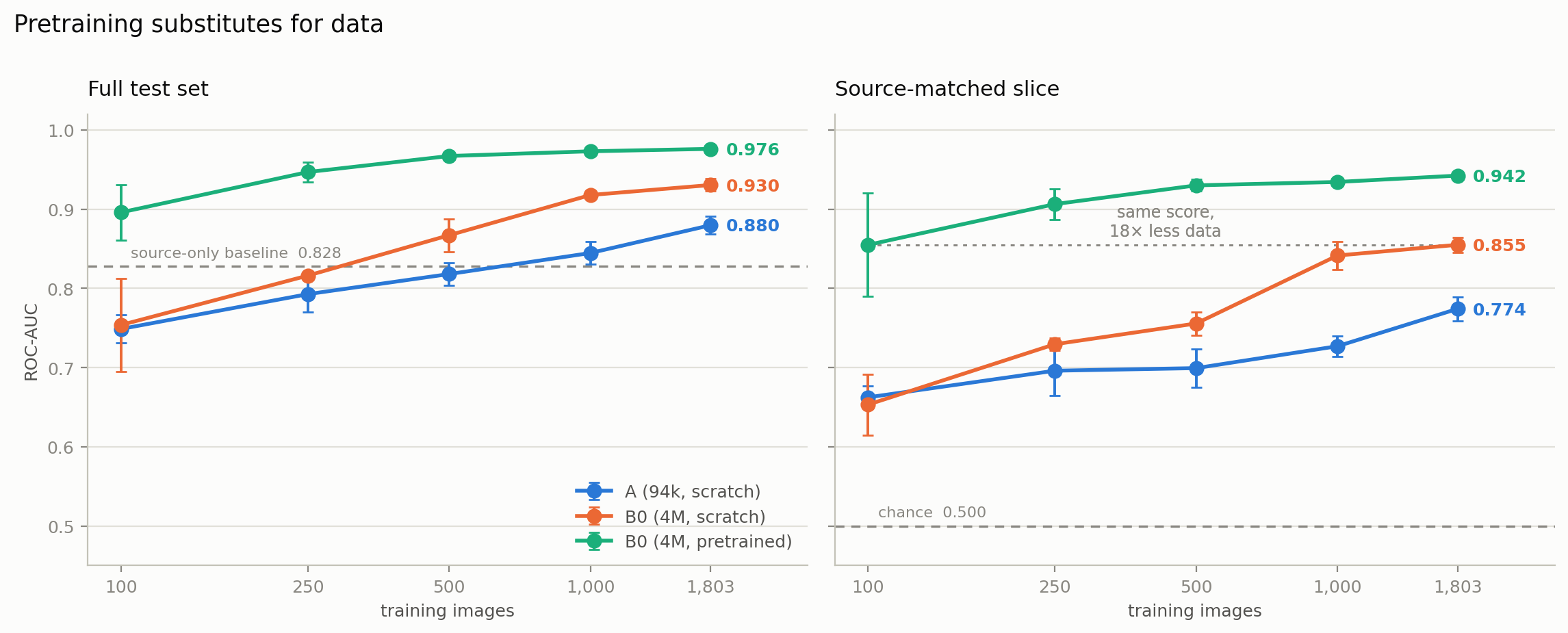
ROC-AUC vs training-set size, three seeds per point, error bars ±1 std. Left: the full test set, with the 0.828 source-only baseline as a dashed line. Right: the source-matched slice, where chance is 0.500.
Pretrained B0 on 100 images scores 0.855. B0-scratch on 1,803 images scores 0.855. Identical architecture, identical score, 18 times the data. In short, pretraining bought an 18× data multiplier.
Pretrained B0 on 100 images also beats my custom CNN trained on all 1,803 (0.774).
We only got that 48/52 split because we looked at the entire dataset.
| training images | 100 | 250 | 500 | 1000 | 1803 |
|---|---|---|---|---|---|
| architecture effect | −0.009 | +0.034 | +0.057 | +0.115 | +0.081 |
| pretraining effect | +0.202 | +0.177 | +0.174 | +0.093 | +0.087 |
At 100 images the 4-million-parameter model is no better than the 94-thousand-parameter one. Capacity is worthless without data to fill it. So at small n, essentially the entire advantage is pretraining, and the pretraining advantage more than doubles as data shrinks.
One more reading of the same curve, which I like because it's blunt. Where does each model cross the 0.828 filename baseline?
| model | images needed to beat a regex |
|---|---|
| B0-pretrained | fewer than 100 |
| B0-scratch | 250–500 |
| my custom CNN | ~1,000 |
how much of the score is provenance (source)?
I defined shortcut reliance as full-test AUC minus source-matched AUC: how much of a model's apparent skill evaporates when source stops being informative.
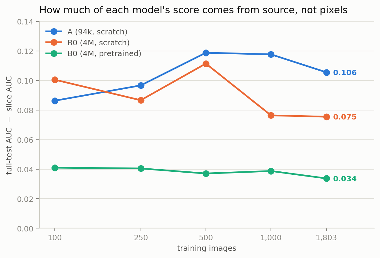
Full-test AUC minus slice AUC, by training-set size. Uncertainty on a difference of two AUCs is roughly ±0.02–0.03, so the wobble in the two scratch arms is noise.
| model | reliance |
|---|---|
| custom CNN | 0.106 |
| B0-scratch | 0.076 |
| B0-pretrained | 0.034 |
The pretrained model leans on the shortcut least, and it's flat across every training size, including n=100, where the provenance (source) rule is nearly a perfect classifier in the training set (only 4 Flickr-negative and 2 Unsplash-positive counter-examples out of 100).
The reading: a model with strong fire-relevant features has no need for the crutch. A weak model takes whatever signal is cheapest, and source detection (filename, photography characteristics, etc) is very cheap.
hard negatives stay hard
Because the source split doubles as a hard/easy negative split, I got a false-alarm breakdown, with no hand-labelling:
| model | clean forests (222 imgs) | sunsets / glare / fog (95 imgs) |
|---|---|---|
| custom CNN | 10% | 42% |
| B0-scratch | 9% | 41% |
| B0-pretrained | 4% | 33% |
The best model false-alarms on a third of the confounders, roughly 8× its rate on easy negatives. And that number is flat across training-set size. More data does not fix hard negatives.
Looking through the confounder images myself, I found sunsets behind ridgelines I myself could not confidently classify at 160 pixels: a diffuse orange band along the horizon with mist in the valley, no plume, no bright core. Is that a sunset or a fire glow?
If I can't tell, some fraction of that 33% isn't model failure at all, it's images where the label is arguable. Without multiple annotators I don't know the human ceiling on this slice, so 33% is an upper bound on the model's error, not a measurement of it. This is also why more data can't help: you can't learn your way out of an ambiguity that exists in the pixels.
the experiment that failed
I planned an experiment where I wanted to fix the shortcut rather than just measure it. So I augmented away the style cue with colour jitter and random grayscale, retrained, and watched the reliance drop.
It made every model worse.
| arm | slice AUC | shortcut reliance |
|---|---|---|
| custom CNN | 0.774 → 0.723 | 0.106 → 0.127 |
| B0-scratch | 0.855 → 0.812 | 0.076 → 0.102 |
| B0-pretrained | 0.942 → 0.934 | 0.034 → 0.036 |
Slice AUC fell across the board and reliance went up for both scratch models, the opposite of what I had predicted.
The results are more obvious in hindsight. *Fire is orange. Stock-photo polish is saturation and contrast.* The shortcut and the signal live in the same channel. There's no colour-space deviation that damages one without damaging the other. So instead of debiasing the model, I took away evidence for the model to classify a fire.
An augmentation can only remove a shortcut that lives in a channel the true signal does not.
Although the experiment did fail, it taught me a new rule to keep with me going forward.
Limitations: I held the epoch budget at 40 while making the task harder, so augmented runs are more under-trained than their controls. Whether it would help at double or triple the budget is untested.
Damage from colour scrambling:
| arm | Δ slice AUC |
|---|---|
| custom CNN | −0.051 |
| B0-scratch | −0.043 |
| B0-pretrained | −0.008 |
The pretrained model is about five times better to colour changes than either scratch model, and B0-scratch is the same architecture, so that's pretraining, not capacity.
Analyzing the change in AUC, I can interpret that the scratch models lean on colour. The pretrained one has shape and texture features that survive when colour is scrambled.
The easier (in theory) fix is to collect negatives from the same source as the positives, so the filenames and photography cues don't give the model hints about how to make its predictions.
small model, big surprise
My last experiment was to test benchmark inference speed, find the fastest model (least MACs), and note any tradeoffs.
My custom CNN has 43x fewer parameters than EfficientNet-B0. It is also slower on CPU with batched input.
Parameters measure storage. MACs (multiply-accumulate operations), measure work. For an anology, parameters are the recipe, MACs are how much you actually do. My custom model runs dense 3x3 convolution filters6 at full spatial resolution (160x160, then 80x80, then 40x40). B0 downsamples hard in its stem and uses depth-wise separable convolutions, which do far less arithmetic per weight.
Measured: 263.8 MMACs for my custom model, 211.5 for B0. The 94k-parameter model does more arithmetic than the 4-million-parameter one.
| my CNN (94k) | B0 (4M) | |
|---|---|---|
| GPU, batch 1 | 0.54 ms | 7.49 ms |
| GPU, batch 32 | 8.39 ms | 19.04 ms |
| CPU, batch 1 | 10.4 ms | 23.2 ms |
| CPU, batch 32 | 465 ms | 408 ms |
| on disk | 0.38 MB | 16.31 MB |
- Compute-bound (CPU, batch 32): latency tracks MACs. I do 25% more arithmetic and run 14% slower. B0 wins.
- Launch-bound (GPU, batch 1): nothing is compute-bound. B0 issues hundreds of small sequential kernels; mine issues about a dozen. 14× faster.
Parameter count does not play a part in either bounds. "Small model = fast model" is a very common wrong assumption in applied ML, and this test was to prove model speed.
The deployment case for the small model is model size and single-image latency.
Lastly, convergence speed measures how fast (in how many epochs) a model learns enough to reach a specific performance threshold. In my experiment, the threshold was set to 0.90 validation ROC-AUC.
| Model Arm | Epochs to Reach Threshold (3 Seeds) |
|---|---|
| B0-pretrained | `[2, 1, 1]` |
| B0-scratch | `[16, 13, 13]` |
| Custom CNN | `[35, None, None]` |
Key Takeaways:
- Pretraining doesn't just improve final accuracy, it reduces the training epoch budget required to reach high performance by .
- Comparing B0-scratch to Custom CNN shows that a well-designed architecture5 converges reliably across random seeds, whereas simple CNNs struggle to optimize on small vision datasets with few epochs to converge.
what i got wrong
A compilation of the predictions I made and their outcomes. It's not flattering, but it's important to note so I can learn from them.
| prediction | outcome |
|---|---|
| Pretraining advantage is largest at small n | held — +0.202 at n=100 vs +0.087 at full data |
| Near-duplicate leakage is a material problem | refuted — 0.7% of test images |
| Shortcut reliance gets worse at small n | refuted — flat across all sizes |
| Overfitting only shows up at small n | refuted — showed at full data as soon as capacity was large |
| Colour augmentation reduces shortcut reliance | refuted — it increased it |
| Augmentation lowers full-test AUC | held |
| The small model is faster | partly — 14× at batch-1 GPU, slower on CPU at batch 32 |
Two held, four refuted, one partial.
The overfitting one I was surprised with. I expected overfitting to be a small dataset problem. It isn't, it's a capacity relative to dataset problem. At full data the final train/val loss gaps were 0.04 / 0.29 / 0.04 for my CNN, B0-scratch and pretrained B0.
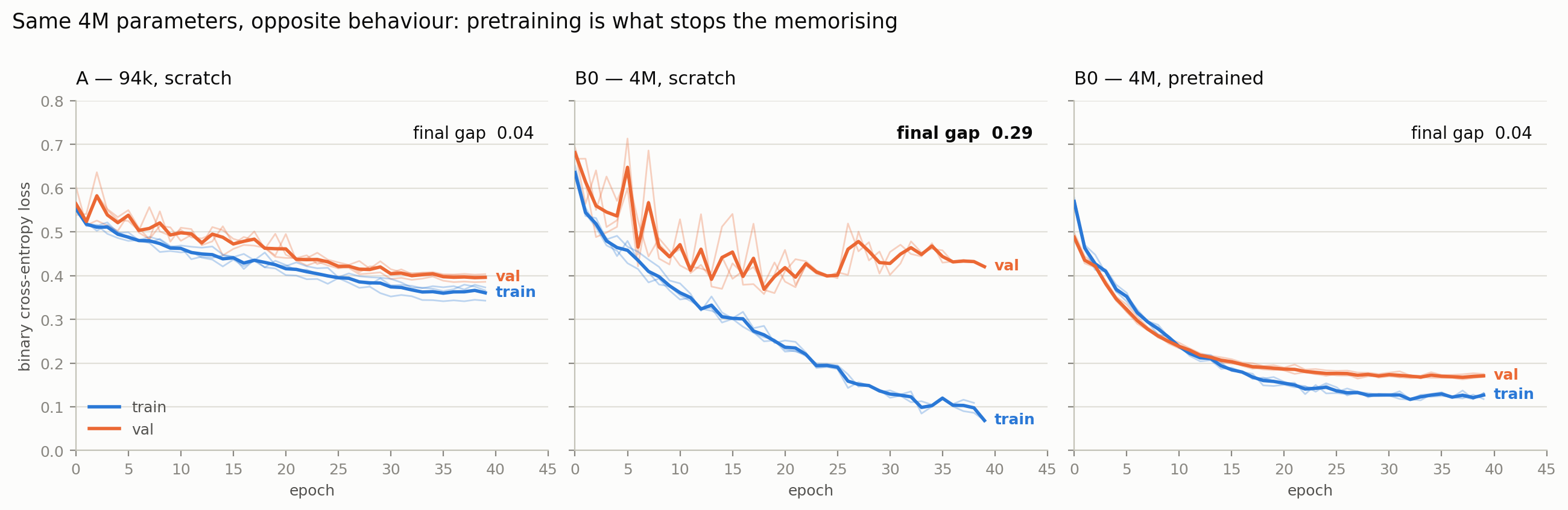
Train and validation loss at full data. Centre: 4M parameters memorising 1,803 images, training loss reaches 0.07 while validation stalls near 0.42. Right: the identical architecture with pretrained weights, gap back to 0.04.
Note that the two 0.04s mean opposite things. My custom CNN sits at 0.36/0.40 with both curves still descending: that's underfit, it ran out of budget before it ran out of learning. Pretrained B0 sits at 0.13/0.17 and flat: that's well fit. The gap alone is a misleading statistic; you need the absolute level too.
the big-picture takeaway
Auditing took more time than I enjoyed. But, ultimately, it decided what dataset to use, how to split it, what to evaluate on, and made me think of what experiments to test. My analysis changed everything downstream of it.
The three things I'd tell myself at the start:
- Report the baseline. Here that was a filename rule at 92.4%. Without it, "90+% accuracy" sounds like an achievement.
- Add the control arm. Without my B0-scratch CNN as a control between the pretraining and architecture of EfficientNet, it would have been impossible to deduce how EfficientNet was better, and the numbers to back it up.
- Publish the failures. The augmentation experiment was humbling, but an interesting outcome to something I was originally so confident would make my models improve.
This is not a deployable wildfire detector. It's an account of what three models learned, why, and where each of them breaks.
I started this project after witnessing the effects of the wildfire spread in Canada. The losses of my people can't be brought back, and although this project isn't a solution to the modern wildfire spread in my country, it taught me lots of how first responders need to be able to evaluate a fire based on what evidence they have (drone footage, planes, pictures, etc).
reproducibility
All training was done on a single Tesla T4 via Kaggle notebooks. Every figure and table traces to a committed CSV and a committed notebook. The split itself is a committed CSV, so every experiment reads the identical train/val/test assignment.
Code and data splits on GitHub
resources
- CBC News. Wildfires and climate change study. CBC News; 2024. Available from: https://www.cbc.ca/news/canada/thunder-bay/wildfires-climate-change-study-9.7297447
- El-Madafri I, Peña M, Olmedo-Torre N. The Wildfire Dataset: Enhancing Deep Learning-Based Forest Fire Detection with a Diverse Evolving Open-Source Dataset Focused on Data Representativeness and a Novel Multi-Task Learning Approach. Forests. 2023; 14(9):1697. https://doi.org/10.3390/f14091697
- Huda R. parking-lot-classifier. GitHub; 2026. Available from: https://github.com/rayyanshuda/parking-lot-classifier
- Zech JR, Badgeley MA, Liu M, Costa AB, Titano JJ, Oermann EK. Variable generalization performance of a deep learning model to detect pneumonia in chest radiographs: A cross-sectional study. PLOS Medicine. 2018; 15(11):e1002683. https://doi.org/10.1371/journal.pmed.1002683
- Tan M, Le QV. EfficientNet: Rethinking model scaling for convolutional neural networks. International Conference on Machine Learning (ICML). PMLR; 2019:6105–6114. https://doi.org/10.48550/arXiv.1905.11946
- Simonyan K, Zisserman A. Very deep convolutional networks for large-scale image recognition. International Conference on Learning Representations (ICLR). 2015. https://doi.org/10.48550/arXiv.1409.1556